How SpikeInterface Handles Time

Extracellular electrophysiology commonly involves synchronization of events across many timestreams. For example, an experiment may involve displaying stimuli to an animal and recording the stimuli-evoked neuronal responses. Accurate timing representation is critical for proper synchronization during analysis.

This tutorial explores how SpikeInterface stores time information and how to use it in your analysis to ensure spike event timing is accurate.

Prerequisites:

A basic understanding of digital sampling (e.g., sampling frequency) is assumed. For a refresher, review the explanation below.

Digital Sampling

What we are fundamentally interested in is recording the electrical waveforms found in the brain. These ‘continuous’ signals change over time. To represent them in finite-memory computers, we sample the continuous signals at discrete points in time.

When sampling, a key question is: How fast should we sample the continuous data? We could sample the signal every \(N\) seconds. For instance, if we sample 4 times per second, this is called the ‘sampling frequency’ (\(f_s\)), expressed in Hertz (Hz), or samples per second.

An alternative way to think of this is to ask: How often do we sample the signal? In this example, we sample every 0.25 seconds, which is called the ‘sampling step’ (\(t_s\)), the inverse of the sampling frequency.

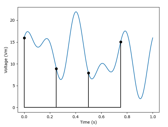
In real-world applications, signals are sampled much faster. For example, Neuropixels samples at 30 kHz (30,000 samples per second) with a sampling step of \(\frac{1}{30000} \approx 0.0000333\) seconds.

Computers typically represent time as a long array of numbers, referred to here as a ‘time array’ (e.g., [0, 0.25, 0.5, 0.75, ...]).

Overview of Time Representations in SpikeInterface

When you load a recording into SpikeInterface, it is associated with a time array. Depending on the data format, this may be loaded from metadata. If no time metadata is available, times are automatically generated based on the sampling rate and the number of samples.

import spikeinterface.full as si

# Generate a recording for this example
recording, sorting = si.generate_ground_truth_recording(durations=[10], seed=0)

# Print recording details
print("Number of samples:", recording.get_num_samples())
print("Sampling frequency:", recording.get_sampling_frequency())
print("Time vector:", recording.get_times())

Number of samples: 250000
Sampling frequency: 25000.0
Time vector: [0.00000e+00 4.00000e-05 8.00000e-05 ... 9.99988e+00 9.99992e+00
 9.99996e+00]

Retrieving information about times

In this example, no time metadata was associated with the recording, so a default time array was generated based on the number of samples and sampling frequency. The time array starts at 0 seconds and continues to \(10 - 1/f_s\) seconds (where \(f_s\) is the sampling frequency), in steps of \(1/f_s\). The recording duration is 10 seconds.

There are a number of helper functions we can use to get information about the times of a recording including:

print("Full time array (s):", recording.get_times())  # note: this will load the entire time array in memory
print("Sliced time array (s):", recording.get_times(start_frame=50, end_frame=100))
print("Start time (s):", recording.get_start_time())
print("End time (s):", recording.get_end_time())
print("Duration (s):", recording.get_duration())

Full time array (s): [0.00000e+00 4.00000e-05 8.00000e-05 ... 9.99988e+00 9.99992e+00
 9.99996e+00]
Sliced time array (s): [0.002   0.00204 0.00208 0.00212 0.00216 0.0022  0.00224 0.00228 0.00232
 0.00236 0.0024  0.00244 0.00248 0.00252 0.00256 0.0026  0.00264 0.00268
 0.00272 0.00276 0.0028  0.00284 0.00288 0.00292 0.00296 0.003   0.00304
 0.00308 0.00312 0.00316 0.0032  0.00324 0.00328 0.00332 0.00336 0.0034
 0.00344 0.00348 0.00352 0.00356 0.0036  0.00364 0.00368 0.00372 0.00376
 0.0038  0.00384 0.00388 0.00392 0.00396]
Start time (s): 0.0
End time (s): 9.99996
Duration (s): 10.0

Shifting the Start Time

You may want to change the start time of your recording. This can be done using the shift_times() method, which adds an offset in seconds to all timestamps in place.

recording.shift_times(100.15)
print(recording.get_times())  # Time now starts at 100.15 seconds

recording.shift_times(-50.15)
print(recording.get_times())  # Time now starts at 50 seconds

[100.15    100.15004 100.15008 ... 110.14988 110.14992 110.14996]
[50.      50.00004 50.00008 ... 59.99988 59.99992 59.99996]

Retrieving Timepoints from Sample Index

SpikeInterface also provides methods to convert between time points and sample indices.

sample_index = recording.time_to_sample_index(58.0)
print("Sample index:", sample_index)

timepoint = recording.sample_index_to_time(50000)
print("Time (s):", timepoint)

Sample index: 200000
Time (s): 52.00000000000001

Manually Setting a Time Vector

It is also possible to manually set a time vector on your recording. This can be useful if you have true sample timestamps that were not loaded from metadata. The benefit of the full time vector is it can include small sampling rate drifts that are not captured when computing the time from the number of samples and sampling frequency alone.

import numpy as np

fs = recording.get_sampling_frequency()

times = 50 + np.arange(recording.get_num_samples()) / fs  # Starts at 50 seconds

# Add some drift to the sampling frequency
drift = np.cumsum(np.linspace(0, 0.001 / fs, recording.get_num_samples()))

true_times = times + drift

recording.set_times(true_times)
print(recording.get_times())

[50.         50.00004    50.00008    ... 60.00487992 60.00491996
 60.00496   ]

The reset_times() method can be used to discard all changes to the start time and remove any time vector on the recording. After reset_times(), times are automatically generated from the sampling frequency, and the start time is zero.

Warning

If your time vector is regularly sampled at the recording’s sampling frequency, and you want to change the start time, it is always better to shift the default times rather than set your own time vector, to save memory.

Multi-segment times

For multi-segment recordings, each segment will have its own timestamps and start time. The methods to interact with times on these segments are the same, but the segment_index must be passed for a multi-segment recording.

recording_segments = si.generate_recording(durations=[10, 20], t_starts=[0, 20])

print("First segment start (s):", recording_segments.get_start_time(segment_index=0))
print("Second segment start (s):", recording_segments.get_start_time(segment_index=1))
print("First segment duration (s):", recording_segments.get_duration(segment_index=0))

First segment start (s): 0
Second segment start (s): 20
First segment duration (s): 10.0

get_total_duration() sums the segment durations, excluding gaps between segments.

print("Total duration (s):", recording_segments.get_total_duration())

Total duration (s): 30.0

Sorting Times

The sorting can also have unique times attached to it. By default, it will inherit the times of the attached recording. However, edits can be made to the times directly on the sorting.

For example, sorting.shift_times() shifts the sorting start time. Note that shifting the recording after registration does not automatically apply the same shift to the sorting.

sorting.register_recording(recording)

sorting.shift_times(1.0)

print("Sorting start time (s):", sorting.get_start_time())
print("Recording start time (s):", recording.get_start_time())

Sorting start time (s): 51.0
Recording start time (s): 50.0

By default, spike trains are returned as sample indices. Using return_times=True returns spike times in seconds. Here we show the first five spike times:

unit_id_to_show = sorting.unit_ids[0]
print(sorting.get_unit_spike_train(unit_id_to_show, return_times=True)[:5])

[51.04260009 51.11048061 51.11576067 51.11992072 51.15840125]

If we shift the sorting by -51 seconds so its start time is zero, the spike times are adjusted accordingly:

sorting.shift_times(-51.0)
print(sorting.get_unit_spike_train(unit_id_to_show, return_times=True)[:5])

[0.04260009 0.11048061 0.11576067 0.11992072 0.15840125]

Aligning Events Across Timestreams

Aligning electrophysiology recordings with other data streams (e.g., behavioral data) is an important step in analysis. This is often done by acquiring a synchronization pulse on an additional channel.

While SpikeInterface does not include built-in features for time-alignment, these resources may be helpful:

• SpikeGLX User Manual

• OpenEphys Synchronization Guide

• NWB Temporal Alignment