Inter-spike-interval (ISI) violations (isi_violation, rp_violation)
Calculation
Neurons have a refractory period after a spiking event during which they cannot fire again. Inter-spike-interval (ISI) violations refers to the rate of refractory period violations (as described by [Hill]).
We aim to calculate the contamination rate \(C\), measuring the ratio of isi violations in the spike-train of a unit. The calculation works under the assumption that the contaminant events happen randomly or come from another neuron that is not correlated with our unit. A correlation will lead to an overestimation of the contamination, whereas an anti-correlation will lead to an underestimation.
Different formulas have been developed, but all require:
\(T\) the duration of the recording in seconds.
\(N\) the number of spikes in the unit’s spike train.
\(t_r\) the duration of the unit’s refractory period in seconds.
Calculation from the [UMS] package
Originally implemented in the rpv_contamination calculation of the UltraMegaSort2000 package: https://github.com/danamics/UMS2K/blob/master/quality_measures/rpv_contamination.m.
In this method the number of spikes whose refractory period are violated, denoted \(n_v\), is used.
Here, the refactory period \(t_r\) is adjusted to take account of the data recording system’s minimum possible refactory period. E.g. if a system has a sampling rate of \(f \text{ Hz}\), the closest that two spikes from the same unit can possibly be is \(1/f \, \text{s}\). Hence the refactory period \(t_r\) is the expected biological threshold minus this minimum possible threshold.
The contamination rate is calculated to be
Calculation from the [Llobet] paper
In this method the number spikes which violate other spikes’ refractory periods, denoted \(\tilde{n}_v\), is used.
The estimated contamination \(C\) is calculated in 2 extreme scenarios. In the first, the contaminant spikes are completely random (or come from an infinite number of other neurons). In the second, the contaminant spikes come from a single other neuron. In these scenarios, the contamination rate is
Where \(TP\) is the number of true positives (detected spikes that come from the neuron) and \(FP\) is the number of false positives (detected spikes that don’t come from the neuron).
Expectation and use
ISI violations identifies unit contamination - a high value indicates a highly contaminated unit. Despite being a ratio, the contamination can exceed 1 (or become a complex number in the [Llobet] formula). This is usually due to the contaminant events being correlated with our neuron, and their number is greater than a purely random spike train.
Example code
Without SpikeInterface:
spike_train = ...   # The spike train of our unit
t_r = ...           # The refractory period of our unit
n_v = np.sum(np.diff(spike_train) < t_r)

# Use the formula you want here
With SpikeInterface:
import spikeinterface.qualitymetrics as sqm

# Combine sorting and recording into sorting_analyzer

isi_violations_ratio, isi_violations_count = sqm.compute_isi_violations(sorting_analyzer=sorting_analyzer, isi_threshold_ms=1.0)
References
UMS implementation (isi_violation)
- spikeinterface.qualitymetrics.misc_metrics.compute_isi_violations(sorting_analyzer, isi_threshold_ms=1.5, min_isi_ms=0, unit_ids=None)
Calculate Inter-Spike Interval (ISI) violations.
- It computes several metrics related to isi violations:
- isi_violations_ratio: the relative firing rate of the hypothetical neurons that are
generating the ISI violations. See Notes.
isi_violation_count: number of ISI violations
- Parameters:
- sorting_analyzerSortingAnalyzer
The SortingAnalyzer object.
- isi_threshold_msfloat, default: 1.5
Threshold for classifying adjacent spikes as an ISI violation, in ms. This is the biophysical refractory period.
- min_isi_msfloat, default: 0
Minimum possible inter-spike interval, in ms. This is the artificial refractory period enforced. by the data acquisition system or post-processing algorithms.
- unit_idslist or None
List of unit ids to compute the ISI violations. If None, all units are used.
- Returns:
- isi_violations_ratiodict
The isi violation ratio.
- isi_violation_countdict
Number of violations.
Notes
The returned ISI violations ratio approximates the fraction of spikes in each unit which are contaminted. The formulation assumes that the contaminating spikes are statistically independent from the other spikes in that cluster. This approximation can break down in reality, especially for highly contaminated units. See the discussion in Section 4.1 of [Llobet] for more details.
This method counts the number of spikes whose isi is violated. If there are three spikes within isi_threshold_ms, the first and second are violated. Hence there are two spikes which have been violated. This is is contrast to compute_refrac_period_violations, which counts the number of violations.
References
Based on metrics originally implemented in Ultra Mega Sort [UMS].
This implementation is based on one of the original implementations written in Matlab by Nick Steinmetz (https://github.com/cortex-lab/sortingQuality) and converted to Python by Daniel Denman.
LLobet implementation (rp_violation)
- spikeinterface.qualitymetrics.misc_metrics.compute_refrac_period_violations(sorting_analyzer, refractory_period_ms: float = 1.0, censored_period_ms: float = 0.0, unit_ids=None)
Calculate the number of refractory period violations.
This is similar (but slightly different) to the ISI violations.
This is required for some formulas (e.g. the ones from Llobet & Wyngaard 2022).
- Parameters:
- sorting_analyzerSortingAnalyzer
The SortingAnalyzer object.
- refractory_period_msfloat, default: 1.0
The period (in ms) where no 2 good spikes can occur.
- censored_period_msfloat, default: 0.0
The period (in ms) where no 2 spikes can occur (because they are not detected, or because they were removed by another mean).
- unit_idslist or None
List of unit ids to compute the refractory period violations. If None, all units are used.
- Returns:
- rp_contaminationdict
The refactory period contamination described in [Llobet].
- rp_violationsdict
Number of refractory period violations.
Notes
Requires “numba” package
This method counts the number of violations which occur during the refactory period. For example, if there are three spikes within refractory_period_ms, the second and third spikes violate the first spike and the third spike violates the second spike. Hence there are three violations. This is in contrast to compute_isi_violations, which computes the number of spikes which have been violated.
References
Based on metrics described in [Llobet]
Examples with plots
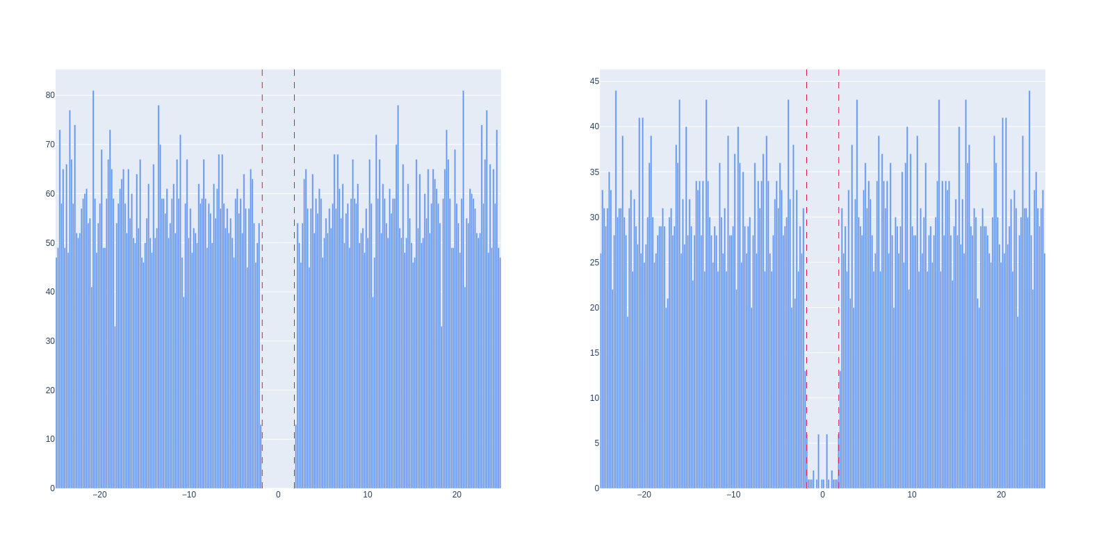
Here is shown the auto-correlogram of two units, with the dashed lines representing the refractory period.
On the left, we have a unit with no refractory period violations, meaning that this unit is probably not contaminated.
On the right, we have a unit with some refractory period violations. It means that it is contaminated, but probably not that much.
This figure can be generated with the following code:
import plotly.graph_objects as go
from spikeinterface.postprocessing import compute_correlograms

# Create your sorting object
unit_ids = ... # Units you are interested in vizulazing.
sorting = sorting.select_units(unit_ids)
t_r = 1.5   # Refractory period (in ms).

correlograms, bins = compute_correlograms(sorting, window_ms=50.0, bin_ms=0.2, symmetrize=True)

fig = go.Figure().set_subplots(rows=1, cols=2)

fig.add_trace(go.Bar(
    x=bins[:-1] + (bins[1]-bins[0])/2,
    y=correlograms[0, 0],
    width=bins[1] - bins[0],
    marker_color="CornflowerBlue",
    name="Non-contaminated unit",
    showlegend=False
), row=1, col=1)
fig.add_trace(go.Bar(
    x=bins[:-1] + (bins[1]-bins[0])/2,
    y=correlograms[1, 1],
    width=bins[1] - bins[0],
    marker_color="CornflowerBlue",
    name="Contaminated unit",
    showlegend=False
), row=1, col=2)

fig.add_vline(x=-t_r, row=1, col=1, line=dict(dash="dash", color="Crimson", width=1))
fig.add_vline(x=t_r, row=1, col=1, line=dict(dash="dash", color="Crimson", width=1))
fig.add_vline(x=-t_r, row=1, col=2, line=dict(dash="dash", color="Crimson", width=1))
fig.add_vline(x=t_r, row=1, col=2, line=dict(dash="dash", color="Crimson", width=1))

fig.show()
Links to original implementations
Literature
Introduced in UltraMegaSort2000 [UMS] (2011). Also described by [Llobet] (2022)